

For some time now an engaged Luxembourg crew is working on the development of a museum of historical calculators and computers. While gathering, repairing and exposing hardware material certainly is the major part of the work, explaining and demonstrating algorithms and software -and identifying their authors- probably is the most exciting activity.
As a special contribution to the Computarium this page wants to show the fastest way of calculating the square-root of a number. I worked it out after the last Computarium exhibition, where we showed how to compute the square-root with paper and pencil or with Napier bones. Today, most people have no clue anymore how to do this, although there are plenty of excellent related web-sites. Among these you'll find an astonishing alternative method that you should consult before continuing these lines: (Although the pages are written in German, they will be easily understood by the excellent graphics. If the German frightens you, please have a look at the graphically awful Square Roots by Pencil and Paper page in English.)
Traditional method:
Toepler's method:
The proof of the correctness of this method is so trivial, that we leave it to the reader. Important note: in base 2 the multiplication by 2 is equivalent to a logical left shift. The obvious advantage of the algorithm is that there is no multiplication and no division. In order to turn this method into an efficiently running procedure, we should consider the operation a bit differently. The next picture shows more evidently that the 1 walks through the steps, while being shifted two digits to the right at each iteration. If at start the result is aligned to the left-most digit -initialized with zero- and each run shifted to the right one digit, then at the end of the algorithm the result must necessarily be correctly right justified. This practice reduces the number of operations and makes the major difference between this algorithm and Rolfe's.
Suppose that our initial argument is 8-bit wide. A computer program then could be written in pseudo-code:
byte x=b'10101001'            //=0xA9
byte res=0                    //start with zero
byte non_shifted_res=0        //idem
byte one=b'01000000'          //=0x40
byte tmp                      //temporary variable
                              //now iterate
REPEAT
tmp=non_shifted_res OR one    //bit operation
non_shifted_res=res           //
IF x>=tmp THEN                //compare
  BEGIN
    x=x-tmp                   //subtract
    non_shifted_res+=one      //add "one" to result
  END
res=non_shifted_res>>1        //shift res 1 digit to the right
one=one>>2                    //shift "one" 2 digits to the right
UNTIL one=1                   //finish
                              //SQRT(x) now is in non_shifted_res
A 32-bit version in H8/3292 Assembler looks like (this could be made faster, if the most frequently used variable was placed in r1r2) :
// fast integer sqrt(x)
// RCX H8/3292
// Abacus algorithm
// Author: Claude Baumann 10/06/2009
// data size U32
// argument x must be in r5r6
// result also is in r5r6
// code generated with Ultimate ROBOLAB v.151
// based on the program "sqrt_integer.vi"
// manually optimized:
// - added "%d" to each label in order to allow multiple macro uses (needs numbers then)
// - OR and SHLR calls replaced by direct operations
// - replaced zero test with faster one
// - masked all superfluous moves as comments
// - masked first subroutine label and final rts 0 as comment
// - removed "_ST_100" from variable names
// - added more comments
//*************************************************************************************
label_sub_fast_square_root
              // make room for stack variables
              mov.w #0x14,r0
              sub.w r0,r7
              // X = argument
              mov.w r5,@(0x0,r7)
              mov.w r6,@(0x2,r7)
              // RES = 0
              mov.w #0x0,r5
              mov.w #0x0,r6
              mov.w r5,@(0x4,r7)
              mov.w r6,@(0x6,r7)
              // NON_SHIFTED_RES = 0
              mov.w #0x0,r5
              mov.w #0x0,r6
              mov.w r5,@(0x8,r7)
              mov.w r6,@(0xA,r7)
              // ONE = 0x40000000
              mov.w #0x4000,r5
              mov.w #0x0,r6
              mov.w r5,@(0xC,r7)
              mov.w r6,@(0xE,r7)
label beginloop_1006%d
              // IF ONE <> 0
              // mov.w #0x0,r3
              // mov.w #0x0,r4
              mov.w @(0xC,r7),r5
              bne loopdo_1006%d
              mov.w @(0xE,r7),r6
              // sub.w r4,r6
              // subx r3L,r5L
              // subx r3H,r5H
              bne loopdo_1006%d
              jmp endloop_1006%d
label loopdo_1006%d
              // TMP = NON_SHIFTED_RES
              mov.w @(0x8,r7),r5
              mov.w @(0xA,r7),r6
              // mov.w r5,@(0x10,r7)
              // mov.w r6,@(0x12,r7)
              // TMP =TMP OR ONE
              mov.w @(0xC,r7),r3
              mov.w @(0xE,r7),r4
              // mov.w @(0x10,r7),r5
              // mov.w @(0x12,r7),r6
              or r4L,r6L
              or r4H,r6H
              or r3L,r5L
              or r3H,r5H
              mov.w r5,@(0x10,r7)
              mov.w r6,@(0x12,r7)
              // NON_SHIFTED_RES = RES
              mov.w @(0x4,r7),r5
              mov.w @(0x6,r7),r6
              mov.w r5,@(0x8,r7)
              mov.w r6,@(0xA,r7)
              // IF X < TMP (simple if)
              mov.w @(0x10,r7),r3
              mov.w @(0x12,r7),r4
              mov.w @(0x0,r7),r5
              mov.w @(0x2,r7),r6
              sub.w r4,r6
              subx r3L,r5L
              subx r3H,r5H
              bcs true_1007%d
              // X = X - TMP
              mov.w @(0x10,r7),r3
              mov.w @(0x12,r7),r4
              mov.w @(0x0,r7),r5
              mov.w @(0x2,r7),r6
              sub.w r4,r6
              subx r3L,r5L
              subx r3H,r5H
              mov.w r5,@(0x0,r7)
              mov.w r6,@(0x2,r7)
              // NON_SHIFTED_RES = NON_SHIFTED_RES OR ONE
              mov.w @(0xC,r7),r3
              mov.w @(0xE,r7),r4
              mov.w @(0x8,r7),r5
              mov.w @(0xA,r7),r6
              or r4L,r6L
              or r4H,r6H
              or r3L,r5L
              or r3H,r5H
              mov.w r5,@(0x8,r7)
              mov.w r6,@(0xA,r7)
label true_1007%d
              // RES = SHLR(NON_SHIFTED_RES)
              mov.w @(0x8,r7),r5
              mov.w @(0xA,r7),r6
              shlr r5h
              rotxr r5L
              rotxr r6H
              rotxr r6L
              mov.w r5,@(0x4,r7)
              mov.w r6,@(0x6,r7)
              // ONE =SHLR(ONE)
              mov.w @(0xC,r7),r5
              mov.w @(0xE,r7),r6
              shlr r5h
              rotxr r5L
              rotxr r6H
              rotxr r6L
              // mov.w r5,@(0xC,r7)
              // mov.w r6,@(0xE,r7)
              // ONE =SHLR(ONE)
              // mov.w @(0xC,r7),r5
              // mov.w @(0xE,r7),r6
              shlr r5h
              rotxr r5L
              rotxr r6H
              rotxr r6L
              mov.w r5,@(0xC,r7)
              mov.w r6,@(0xE,r7)
              jmp beginloop_1006%d
label endloop_1006%d
              mov.w @(0x8,r7),r5
              mov.w @(0xA,r7),r6
              // free stack variable space
              mov.w #0x14,r0
              add.w r0,r7
              // end_of_sub_fast_square_root
              // rts 0
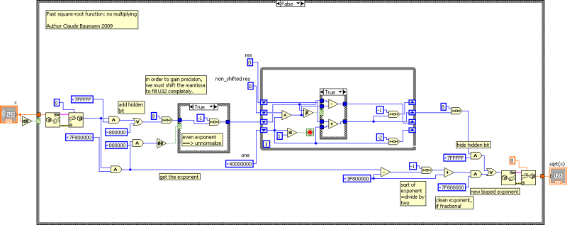
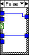
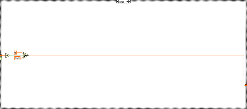
A 32-bit version would have the following aspect in LabVIEW:
The algorithm not only works for integer values, but may easily be used with floating point numbers. Here a simple LabVIEW version for IEEE standard single precision floating point data. There are three important tricks to observe here. First, the program must expand the argument and later normalize the result. Now the mantissa may be considered as an integer. Finally the exponent must simply be divided by two. In the case of an initially even exponent, the mantissa must be shifted one digit to the right before operation.
![]()
![]()
An ULTIMATE ROBOLAB version for long unsigned integer looks like:
- Ralph Hempel recommends the excellent book: Jack. W. Crenshaw, Math Toolkit for Real-Time Programming, CMP Books, Lawrence KS, USA, 2000
- How ENIAC specialists thought about the square-root in 1949.
- ARM code square root routines
- Other Abacus method
- How Zuse computed the square-root on the Z3 in 1941
- Historic calculators
- Toepler Verfahren (German)
- M. Gärtner's Artikel üver das Toepler Verfahren (German)
- Berechnung der Quadratwurzel (German); has an extract of Friden's patent